

Probabilities & Distribution Functions - Machine Learning
Insights on PDF, CDF and many more...

Probability in simple terms…
Likelihood of occurrence of a random event.
The chance that a given event will occur.
Addition Rule
Mutually Exclusive Events
P(A or B) = P(A) + P(B)
e.g. Probability of getting H or T after tossing a coinNon Mutually Exclusive Events
P(A or B) = P(A) + P(B) — P(A and B)
e.g. Probability of picking a King & Heart from a deck of cards
Multiplication Rule
Independent Events— Two events are independent if they do not affect one another.
P(A and B) = P(A) * P(B)
e.g. Tossing a coin, Rolling a diceDependent Events— Two events are dependent if they affect each other
P(A and B) = P(A) * P(B/A) [conditional probability or Naive Baye’s]
e.g. Take a King card from deck (4/52) without putting it back and then pull a Queen card from the same deck (4/51)
Probability Distribution Function
PDF describes how the probabilities are distributed over the values of a random variable.
Types
1. Probability Mass Function (PMF): Used for discrete random variables
2. Probability Density Function (PDF): Used for Continuous random variables
3. Cumulative Distribution Function (CDF): Used for both Discrete (PMF) and Continuous (PDF) variables and is the cumulative representation of it.
PMF — Probability Mass Function
e.g. Rolling a dice {1,2,3,4,5,6} i.e. a fair dice
=> P(1) = P(2) = P(3) = P(4) = P(5) = P(6) = 1/6
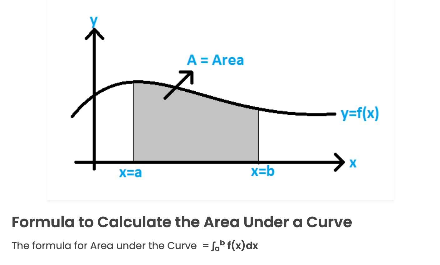
PDF — Probability Density Function
It defines the probability function representing the density of a continuous random variable lying between a specific range of values.
Area under the curve: The area under a curve between two points is found out by doing a definite integral between the two points.
Probability density: a statistical measure used to gauge the likelihood that an event will fall within a range of continuous values.
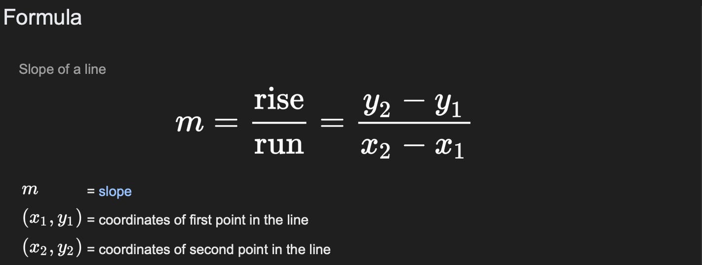
-> Slope of the point or Gradient of cumulative curve or CDF.
Properties:
1. Non-negative f(x) ≥ 0 for all x
2. The total area under the PDF curve is equal to 1 i.e. f(x) dx = 1
3. W.r.t different distributions, f(x) function is going to change.
Cumulative Distribution Function (CDF)
It's the cumulative sum of all the probabilities which we got via PMF or PDF
Value ranges between 0 to 1.
Represented by sigmoid curve
Types of Distribution
Bernoulli Distribution
It is the simplest discrete probability distribution and PMF is used.
It represents the probability distribution of a random variable that has exactly two possible outcomes, i.e. Binary Outcomes
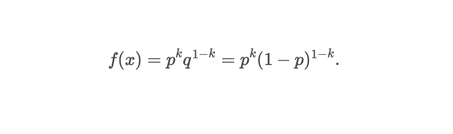
Success (1) → with probability p| Failure (0) → with probability 1-p
e.g. Tossing a coin {H, T}
P(H) = 0.5
P(T) = 1 — P(H) = 0.5PMF formula:
Mean: E(x) = ∑ k * P(k), where k = {0, 1}
E(x) = p (where k=1)Median:
= 0 if p < 1/2
= 0.5 if
Binomial Distribution
The Binomial Distribution with parameters n and p is the discrete probability distribution of the number of successes in a sequence of n independent experiments, each asking a yes-no question, and each with its own Boolean-valued outcome: success (with probability p) or failure (with probability q = 1-p).
A single success/failure experiment is also called a Bernoulli trial or Bernoulli experiment.
A sequence of outcomes is called a Bernoulli process.
Binomial Distribution is a combination of a group of Bernoulli distribution in sequence whose outcomes are either 0’s or 1's.
It works with Discrete Random Variable
Every outcome of the experiments is Binary i.e. 0 or 1.
All the experiments are performed for n trials
Denoted by B(n,p), where n ⍷ {0, 1, 2,….} => No. of trials or experiments
Support Parameter: K ⍷ {0, 1, 2,….n} => No. of successes
PMF:
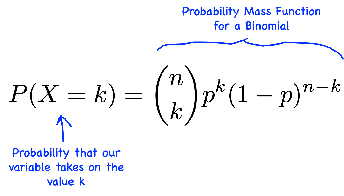
where C (n, k) = n! / (k! (n-k)!). => Also called as Binomial Coefficient
Mean: n * p
Variance: n* p* q
Standard Deviation: sqrt (n*p*q)
Poisson Distribution
Is is a discrete probability distribution that expresses the probability of a given number of events occurring in a fixed interval of time if these events occur with a known constant mean rate and independently of the time since the last event.
Discrete Random Variable and PMF is used
Describes the number of events occurring in a fixed time intervals
e.g. No. of people visiting banks every hourPMF:
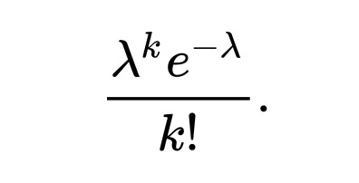
where λ is the number of events at every time interval
and k is the number of occurrencesMean & Variance: E(x) = ƛ * t
where ƛ is the number of events occur at every time interval
and t is the time interval
Normal / Gaussian Distribution
It is a type of continuous probability distribution for a real-valued random variable.
Continuous Random Variable and will use PDF
It follows a Bell Curve which denotes Mean = Median = Mode
It also follows Symmetric distribution
As variance increases, the spread of the data also increases and vice-versa
PDF:
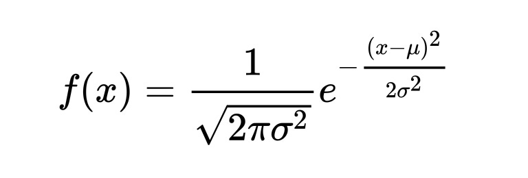
Mean: μ = ∑ (X/n)
Variance: ∑ (X-μ)² /n
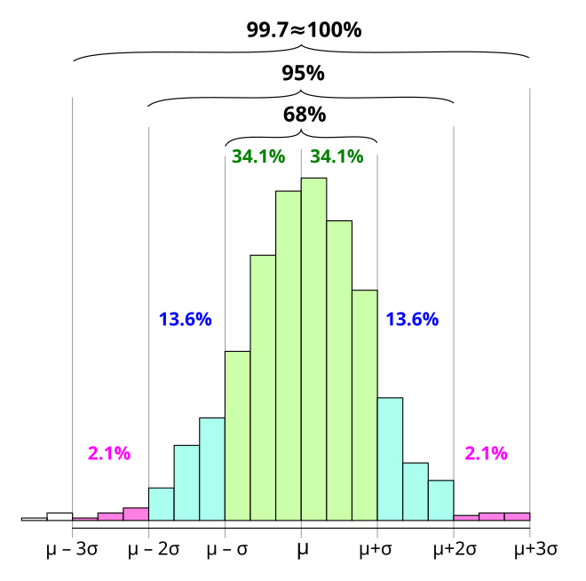
Empirical Rule of Normal/Gaussian Distribution
68–95–99.7 rule, also known as the empirical rule represents the percentage of values that lie within an interval estimate in a normal distribution.
=> 68% of the value lie within 1 SD of the mean
=> 95% of the value lie within 2SD of the mean
=> 99.7% of the values lie within 3 SD of the mean
Standard Normal Distribution
The standard normal distribution is a special case of the normal distribution where μ=0,σ²=1.
If is often essential to normalize data prior to the analysis. A random normal variable with mean μ and standard deviation μ can be normalized via the following:
z- score = (x−μ) / σ
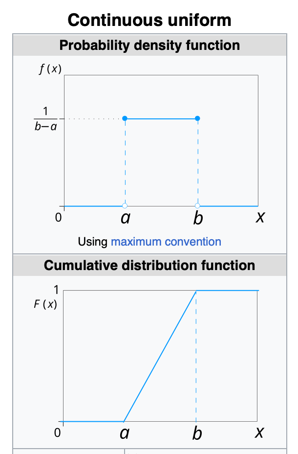
Uniform Distribution
Continuous Uniform Distribution (pdf):
Continuous Uniform Distribution or Rectangular distributions are a family of symmetric probability distributions.
Such a distribution describes an experiment where there is an arbitary outcome that lies between certain bounds.
The bounds are defined by the parameters, a and b which are the minimum and maximum values.
Mean, Median: 1/2 * (a + b)
Variance: 1/12 * (b-a)²
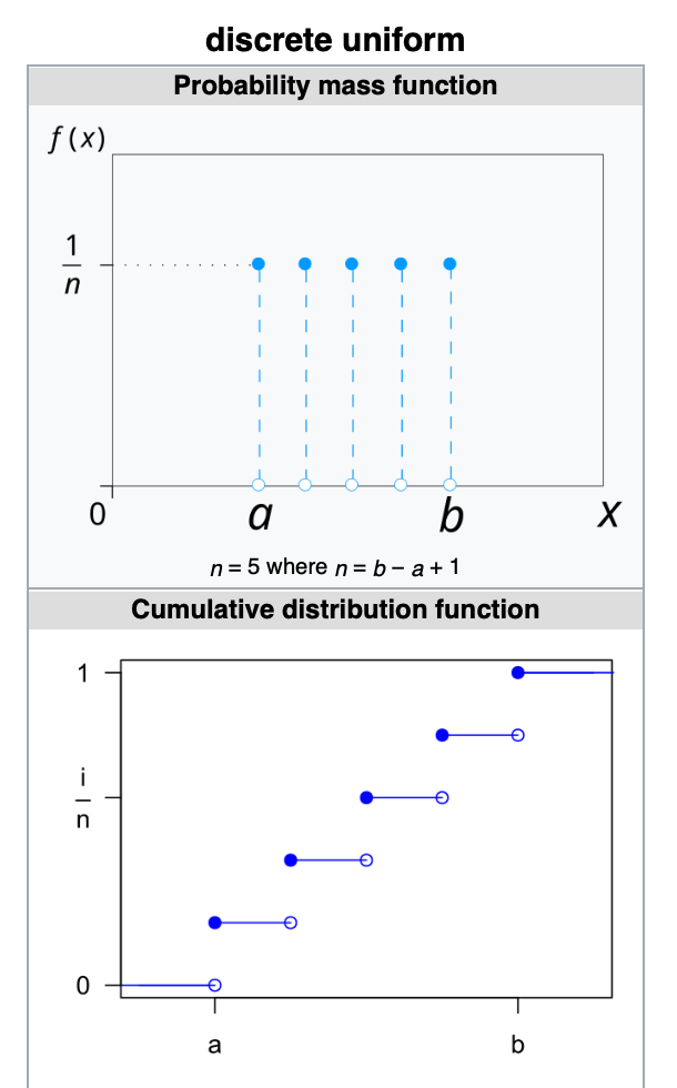
2. Discrete Uniform Distribution (pmf)
Discrete Uniform Distribution is a symmetric probability distribution wherein a finite number of values are equally likely to be observed
Every one of n values has equal probability 1/n
Discrete Uniform Distribution would be a known finite number of outcomes equally likely to happen
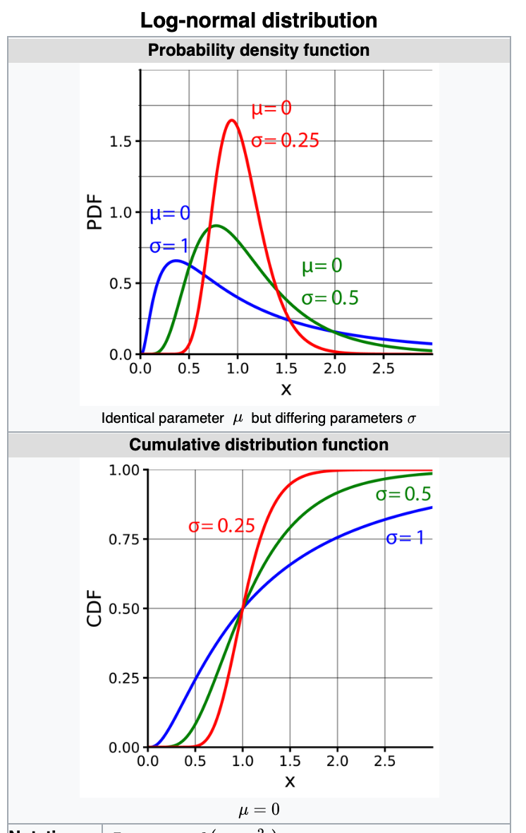
Log Normal Distribution
It's a continuous probability distribution of a random variable where logarithm is normally distributed.
If the random variable X is log-normally distributed, then Y = ln (X) has a normal distribution. [here ln is natural log, i.e. log to the base of e]
Equivalently, if Y has a normal distribution, then X = exp (Y) has a log-normal distribution.
Its a right-skewed distribution. E.g Wealth distribution of the world
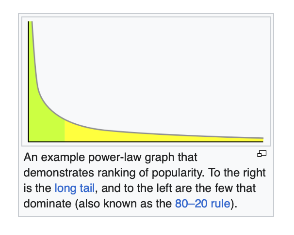
Power Law Distribution [Pareto Distribution]
Power Law Distribution is a functional relationship between two quantities, where a relative change in one quantity results in a proportional relative change in the other quantity, independent of the initial size of those quantities, one quantity varies as a power of another.
Follows 80% — 20% rule i.e. 80 percent of x is in first 20 percent of y.
The idea here is small number vast majority.E.g. In a cricket match, 20% of the team is responsible for winning 80% of the match.
Its a Non-Gaussian Distribution which can be transformed to Normal Distribution using Box-Cox transformation technique.
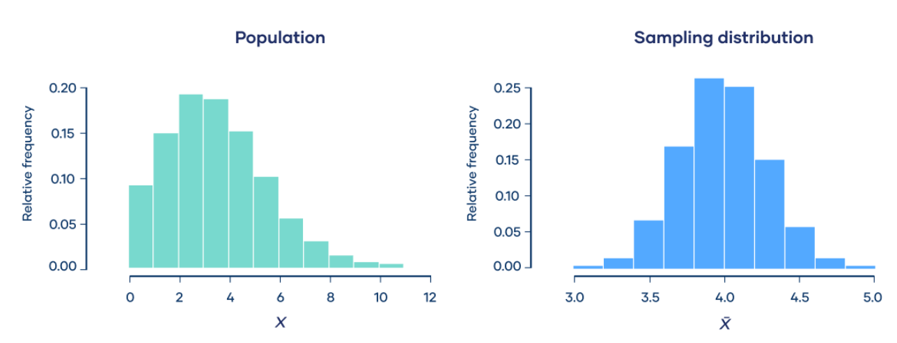
Central Limit Theorem
The central limit theorem says that the sampling distribution of the mean will always be normally distributed, as long as the sample size is large enough.
Regardless of whether the population has a normal, poisson, binomial, or any other distribution, the sampling distribution of the mean will be normal.
Fortunately, you don’t need to actually repeatedly sample a population to know the shape of the sampling distribution. The parameters of the sampling distribution of the mean are determined by the parameters of the population.
Calculation:
The mean of the sampling distribution is the mean of the population.

The standard deviation of the sampling distribution is the standard deviation of the population divided by the square root of the sample size.

We can describe the sampling distribution of the mean using this notation:
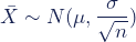
Where:
X̄ is the sampling distribution of the sample means
~ means “follows the distribution”
N is the normal distribution
µ is the mean of the population
σ is the standard deviation of the population
n is the sample size
Sample size and the central limit theorem
The sample size (n) is the number of observations drawn from the population for each sample. The sample size is the same for all samples.
The sample size affects the sampling distribution of the mean in two ways.
1. Sample size and normality
The larger the sample size, the more closely the sampling distribution will follow a normal distribution.
When the sample size is small, the sampling distribution of the mean is sometimes non-normal. That’s because the central limit theorem only holds true when the sample size is “sufficiently large.”
By convention, we consider a sample size of 30 to be “sufficiently large.”
When n < 30, the central limit theorem doesn’t apply. The sampling distribution will follow a similar distribution to the population. Therefore, the sampling distribution will only be normal if the population is normal.
When n ≥ 30, the central limit theorem applies. The sampling distribution will approximately follow a normal distribution.
2. Sample size and standard deviations
The sample size affects the standard deviation of the sampling distribution. Standard deviation is a measure of the variability or spread of the distribution (i.e., how wide or narrow it is).
When n is low, the standard deviation is high. There’s a lot of spread in the samples’ means because they aren’t precise estimates of the population’s mean.
When n is high, the standard deviation is low. There’s not much spread in the samples’ means because they’re precise estimates of the population’s
Estimate
It is specified observed numerical value used to estimate an unknown population parameter.
1. Point Estimate
Single numerical value used to estimate an unknown population parameter.
e.g. Sample mean is point estimate of population mean.
2. Interval Estimate
A range of values are used to estimate an unknown population parameter.
e.g. Alone sample mean doesn’t help us always to estimate the population mean, but sample mean having a range of value will be much better choice, which is also called as confidence interval.
Thank you so much for reading.
If you have any questions or suggestions, leave a comment.
Follow my work on other platforms: